cs766project
Mandarin orange grading using support vector machine classification and transfer learning
Heather Shumaker & Mary Feng
Motivation
The quality of fruit is often associated with its outside appearance. The fruits sold at the grocery store are examined and judged for quality before shipping. Features such as color, size, and shape can affect the way that consumers select fruit and influence market value of produce. In order to make the highest profit, grocery stores sell the best looking fruits to appeal to customers. Fruit grading is an important step in selecting high quality fruit to bring from the farm or orchard to the consumer. Automating the fruit grading process is important for reducing the time and labor compared with the manual process conducted by humans. Computer vision-based techniques for fruit grading are often inexpensive and nondestructive which make them very competitive compared to manual inspection and machine physical inspection.
Current State-of-the-art
Although there are some papers which discuss automated fruit grading techniques using computer vision, implementation of this is more rare in industry. One example is Ellips, which is a Dutch company that uses size and color to determine quality. Compac, a New Zealand-based company, uses software to grade cherries. Many agricultural companies still rely on humans to grade produce. There are some machines available for sorting and grading based on physical characteristics such as shape, weight, and how the fruit rolls. It appears many companies capable of automated visual fruit grading are located outside the United States or work specifically for one kind of fruit.
There are several papers and companies that have implemented computer vision techniques with machine learning for orange grading. This includes classic machine learning algorithms involving some feature engineering, and more recently, deep learning methods for classification.
Project Overview
The goal of this project is to grade the quality of mandarin oranges through computer vision techniques into the categories created by observing international standards. This project began without a certain fruit in mind, however, after a literature review, we decided that mandarin oranges would be a good candidate for this project. Mandarin oranges are readily available to us and have a similar shape from all angles. Additionally, we found two papers that successfully graded oranges through support vector machine (SVM) learning [1] and neural networks [2]. We also found many more papers describing orange imaging and image segmentation techniques. We would like to implement our own versions of SVM and neural networks to determine the best method for grading the oranges.
Grading Scale
The grading scales used in previous research were not based on any national or international standard. In most cases the oranges were given a number between 1 and 5. For this project, we originally decided to roughly follow the USDA tangerine grading standards [3] to group the oranges into 5 categories: US Fancy, US No. 1, US No. 2, US No. 3, and below which we will call US No. 4. However, after testing the two techniques, we reduced the number of classes to three. Since it is difficult for even us, as humans, to distinguish between the five possible classifications, we reduced to three categories: sellable (highest quality, which could be sold at a normal price), discount (medium quality, which would be sold at a discount price), and throwaway (low quality, not to be sold).
Mandarin Orange Imaging
For this project, we wanted to simulate oranges on an assembly line. Unfortunately, there were no large publicly available image sets which were suitable for the purposes of this project. Therefore, we took the images ourselves. Following a process similar to what several papers detailed, the photos were taken in a light box with a black background with the orange in the center. The camera was fixed throughout the images with a known image window size of 0.071 millimeters per pixel. We captured 557 images of about 86 oranges at four different angles each. The images were captured from the top, bottom, and two sides of each orange.
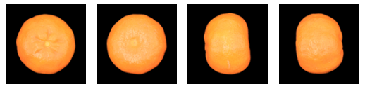
Figure 1. A mandarin orange from the top, bottom, side, and other side.
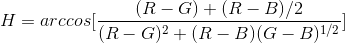
The images were captured with a DSLR camera fixed to a mount with a shutter speed of 1/100, an aperture of f9, a 50mm lens, and an ISO of 1250. A diffused lighting system was used to capture the images to avoid bright spots and reflectance on the surface of the oranges. After the images were acquired, they were preprocessed by removing the background and cropping the images to 1001 by 1001 pixels with the centroid of the orange in the center of the image. The red channel was a good estimate of the mask of the orange and was used to separate the orange from the background.
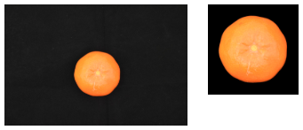
Figure 2. Original image of the orange (left) and cropped image with background removed (right).
Each color channel of the oranges was evaluated for its properties and potential uses. The green channel may be used to determine the quality of the color and segmentation of all defects and the blue channel may be used for segmentation of lighter defects such as scarring on an orange’s skin. The blue channel may also be used for texture analysis. The red channel can be used for segmentation of dark defects.
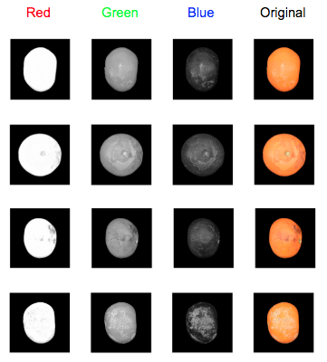
Figure 3. The red, green, and blue channels of the orange photos can be used to detect different defects and discoloration. The red channel was useful for calculating the mask of the oranges.
Training and Testing
To compare traditional machine learning methods and deep learning, the dataset was split into training and test sets. The same training set was used to train models for traditional machine learning techniques and neural networks. The same test set was used to compare accuracy between the final selected traditional machine learning model and final selected neural network.
| Sell | Discount | Throwaway | |
|---|---|---|---|
| Train | 277 | 149 | 42 |
| Test | 15 | 15 | 10 |
Feature Extraction
Shape Features
Following some of the features extracted in [1], we computed the size of each orange. We can compute size using the MATLAB function regionprops on the binarized image. An image was captured with a ruler in the scene to calculate the size of each pixel. Since the pixel size is known and constant through all images, we can compute the area of each orange in mm2. Since the oranges are taken at different angles and some are circular and some are more ellipsoid, we did not compute the roundness of the orange. Instead, we computed the circularity by calculating the perimeter and area of the orange using regionprops and calculating 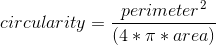 . The circularity was calculated to extract a feature based on the lumpiness of the exterior of the orange. The diameter of the orange was also measured using regionprops.
Color Features
Following the color feature extraction of [1,2] we extracted the mean, standard deviations, and range of the intensity of all three color channels. Additionally, we compute hue, saturation, and intensity (HSI) and the corresponding mean and standard deviations according to:
 The standard deviation of the H value is a good indicator for the maturity of the orange since the histogram of an unripe orange has one peak and a ripe orange has two peaks [1].
Defect Features
A key feature that can be used to determine quality is the percent of blemished skin on the orange. The percent of blemished skin can be computed through image segmentation. Dark spots were identified using the red color channel and thresholded to distinguish dark defects. For defects which were light in color, such as some types of scarring, the blue and green color channels were attempted to be used in a similar method to detecting dark defects. However, it was difficult to distinguish between shine/glare and truly light defects. Therefore, the saturation channel of the HSV color space was used to identify light defects.
The calyx of the orange (the stem portion) can easily be mistaken for a blemish through segmentation. To account for this we have removed blemishes that occur at the centroid of the image if the orange is significantly round (from top view). First, a gaussian blur is applied to each channel to remove possible segments due to texture. The darker blemishes can be measured by looking at the red channel at pixels below the mean image value. Lighter blemishes were identified in a similar fashion, using the saturation channel of the image in HSV color space and thresholding with the mean saturation value times a constant multiplier—0.7 was found to work well empirically. The images were binarized so that the defects had a pixel value of 1 and the rest of the image was 0.
The perimeter of the orange often remained in the binarized image so to eliminate this we subtract a dilated version of the perimeter. The resulting image is dilated slightly to connect components that are very close together. Each segment is labeled using bwlabel and then the segments are looped through to remove the calyx and any remaining portions of the perimeter of the orange. The calyx is removed by checking if a segment is very close to the center of the image, the orange is of sufficient roundness to be on the top view, and the spot is fairly small to consider instances in which there are defects near the calyx. Small components under 40 pixels are removed and line-like components from the remains of the perimeter are removed by checking for roundness. If the roundness is under 0.1, the segment is removed. We can then compute the percent of skin blemished by dark and light spots by dividing the sum of all the remaining pixels divided by the size of the mask.
Figure 4. The red channel can be used for detecting dark blemishes on the oranges. After processing, the pixels can be summed and divided by the sum of the mask.
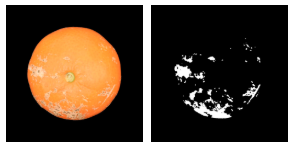
Figure 5. The saturation channel of HSV color space is used to identify light defects. The above left image is the image before processing, and the left image depicts the defects identified result after all processing, including identifying dark and light blemishes and removing the calyx and perimeter.
Texture Features
Characteristics relating to texture are used to capture the roughness or smoothness of the orange peel. Metrics of texture could help with distinguishing between oranges with smooth surfaces, which are more desirable for selling, and those which have rougher, bumpy textures due to blemishes and discolorations. Rough textures feature more variation in intensity values, while smooth textures have less variation in intensity values. Entropy is one measure used to quantify texture; it is a statistical measure of randomness. Higher values indicate rougher textures, while smaller values indicate smoother textures.
Texture analysis is done with the gray-level co-occurrence matrix (GLCM). GLCMs are created by calculating the number of times a pixel with intensity i occurs with a specified spatial relationship to a pixel with intensity j. Various statistics, including contrast, correlation, energy, and homogeneity, can be extracted from the GLCM. For this task, an offset of 5 pixels was used with four directions (angles 0, 45, 90, and 135). This results in four GLCMs and thus four values for each statistic. The mean is taken for each statistic and used as the value in the feature vector. These statistics characterize the texture of the orange peel by measuring the amount of variability of intensity values of pixels in the orange image.
Feature Vector
The resulting feature vector contains the following 24 features:
- Area
- Circularity
- Diameter
- Mean R channel intensity
- Mean G channel intensity
- Mean B channel intensity
- Standard deviation of R channel
- Standard deviation of G channel
- Standard deviation of B channel
- Range of R channel
- Range of G channel
- Range of B channel
- Mean of Hue (H)
- Mean of Saturation (S)
- Mean of Intensity (I)
- Standard deviation of Hue (H)
- Standard deviation of Saturation (S)
- Standard deviation of Intensity (I)
- Percentage of blemished skin
- Entropy
- Contrast
- Correlation
- Energy
- Homogeneity
Traditional Classification Models Considered
Splitting training set into training and validation set
To refine models and predict accuracy, the training set was split into a set for training models and a set for validation. A 70/30 split was done for training and validation, resulting in a set of 329 examples for training and 139 examples for validation. The following models were trained on this training set consisting of 329 examples.
Various classification models were considered and explored for grading oranges with the Classification Learner app in MATLAB. These include decision trees, nearest neighbor classifiers, SVMs, and ensembles. The following chart shows the results using the default settings and 10 fold cross validation. Comparing these various classification models, it appears that SVMs perform quite well, with the best performing models achieving higher accuracy.
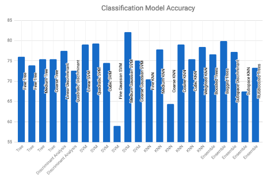
Figure 6. Classification model accuracy using 10-fold cross-validation
The chart below shows results similar to above but only using 6 features (columns 4, 6, 9, 12, 21, 24) as selected by sequential feature selection. The resulting accuracies are comparable to the corresponding accuracies above.
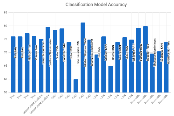
Figure 7. Classification model accuracy with sequential feature selection
Feature Selection
While many features have been extracted, not all may be useful in predicting the quality of an orange. Using too many features and/or keeping features which are irrelevant or redundant may lead to various issues, including overfitting and degrading classifier performance as the number of dimensions increase with each additional feature—the curse of dimensionality. Additionally, fewer features can be desirable as the resulting models could be simpler to interpret and take less time to train. There are a few broad categories of methods to perform feature selection: filter methods, wrapper methods, and embedded methods. Filter methods select features based on a particular measure, such as mutual information or statistical tests of significance. This often used in preprocessing, as features are selected independently of a particular model. On the other hand, wrapper methods use a particular model in selecting subsets of features. A model is trained on a subset of the features and performance is measured on a hold-out set. Since this involves fitting a model for each subset of the features, wrapper methods are more computationally expensive than filter methods. Some common wrapper methods include forward selection and backward elimination. Finally, embedded methods perform feature selection as a part of building a model. For instance, regression models with regularization using Lasso, Ridge, or elastic net penalize more complex models.
As a preprocessing step, filter methods are used for feature selection. Filter methods were used to obtain more insight on which features are most predictive and to prevent potential overfitting using other methods. Two filter methods are considered for feature selection: ReliefF and (forward) sequential feature selection.
ReliefF
The ReliefF algorithm uses k nearest neighbors to determine weights of predictor variables by penalizing variables which are less discriminative and rewarding those which are more discriminative. The default amount of neighbors k = 10 was used; this was empirically found to be a stable value after experimenting with various values of k. The top ten ranked features and associated weights are displayed in the table below.
| Rank | 1 | 2 | 3 | 4 | 5 | 6 | 7 | 8 | 9 | 10 |
|---|---|---|---|---|---|---|---|---|---|---|
| Feature | 6 | 17 | 3 | 1 | 11 | 7 | 19 | 15 | 9 | 20 |
| Weight | 0.0595 | 0.0432 | 0.0397 | 0.0330 | 0.0326 | 0.0316 | 0.0302 | 0.0288 | 0.0285 | 0.0282 |
Table 1. Feature ranking using the ReliefF algorithm
(Forward) Sequential Feature Selection
Sequential feature selection is a popular method of determining important features. Forward searching begins with an empty subset of features and incrementally adds features one at a time until a certain criterion is met. For this task, the criterion used is misclassification error; it is simply the amount of misclassified observations divided by the number of observations. Stratified leave one out cross validation (LOOCV) was used as the validation method to compute the criterion. The results are detailed in the table below.
| Step | Feature Added | Criterion value (misclassification error) |
|---|---|---|
| 1 | 4 | 0.282675 |
| 2 | 6 | 0.234043 |
| 3 | 21 | 0.209726 |
| 4 | 24 | 0.191489 |
| 5 | 12 | 0.18845 |
| 6 | 9 | 0.179331 |
Table 2. Features selected using the Sequential Feature Selection Algorithm.
Support Vector Machine Grading
Based on the performances in the tables above, the final model chosen was a medium Gaussian SVM, with box constraint level 1, kernel scale 2.4, multiclass method of one-vs-one, and the predictor columns were standardized (centered and scaled by their corresponding weighted means and weighted standard deviations).
Two versions of this model were used on the validation set (which was not used in training these models) to assess performance and have an estimate of accuracy; these two versions are with and without feature selection.
The following displays the confusion matrices on the validation set.
| Predicted | ||||
|---|---|---|---|---|
| True class | Sell | Discount | Throwaway | Accuracy |
| Sell | 77 | 6 | 0 | 92.8% |
| Discount | 23 | 21 | 0 | 47.7% |
| Throwaway | 0 | 2 | 10 | 83.3% |
| Average | 77.7% |
Table 3. Validation set confusion matrix without feature selection
| Predicted | ||||
|---|---|---|---|---|
| True class | Sell | Discount | Throwaway | Accuracy |
| Sell | 75 | 8 | 0 | 90.4% |
| Discount | 21 | 23 | 0 | 52.3% |
| Throwaway | 0 | 2 | 10 | 83.3% |
| Average | 77.7% |
Table 4. Validation set confusion matrix with feature selection
Overall, it appears there is not much difference in accuracy between using feature selection and not using feature selection. Therefore, the final model used on the test set used a subset of features (columns 4, 6, 9, 12, 21, 24 as selected by sequential feature selection) in an attempt to pick a simpler model and avoid overfitting. The result on the test set is displayed below.
| Predicted | ||||
|---|---|---|---|---|
| True class | Sell | Discount | Throwaway | Accuracy |
| Sell | 14 | 1 | 0 | 93.3% |
| Discount | 8 | 7 | 0 | 46.7% |
| Throwaway | 0 | 2 | 8 | 80.0% |
| Average | 72.5% |
Table 5. Test set confusion matrix with feature selection
Neural Network Grading
To implement orange grading using a neural network, we used transfer learning to adjust a pre-trained convolutional neural network (CNN) to work for our application. There are several pre-trained networks made to classify orange images. We tested AlexNet and GoogLeNet, two networks trained to classify ImageNet images. MATLAB 2017a has a simple interface with both networks that allowed us to conduct transfer learning with our set of orange images. We sorted the orange photos into folders of each grade. In order to use AlexNet, our images were resized to 227 by 227 pixels using imresize. For GoogLeNet, the images had to be resized to 224 by 224 pixels. Fortunately, both networks work with RGB images so no additional processing will have to be done on the images.
Our first round of transfer learning on AlexNet did not have good results. The validation accuracy of the network with five classes was 27 percent. In order to improve the accuracy of the network, we combined two of the five grades since there is only a slight difference between some of the orange photos. After combining five classes into three classes, the AlexNet model showed a validation accuracy of 72 percent (Figure 8).
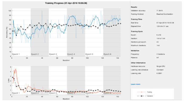
Figure 8. Network evaluation after reducing the categories from 5 to 3.
At this point, GoogLeNet was also trained on the data and showed a similar accuracy of 71 percent. Since the GoogLeNet training took almost twice that of AlexNet, we chose to use the AlexNet model for the rest of the testing. The learning rate was adjusted from 1e-4 to 1e-5 and showed similar results. We also changed the mini-batch slightly but found that a mini-batch size of ten gave good results. Since the training was conducted with only a CPU, we did not have much time to test the training validation accuracy with many different network parameters. However, in attempt to improve the accuracy of both the machine learning and deep learning methods, we added 212 more photos to the training set. Unfortunately, adding the 212 extra photos did not improve the network accuracy (Figure 9). This could be due to the fact that most of the images that were added were of the sellable and discount quality when the network really needed to see more throw away and discount oranges.
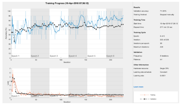
Figure 9. Network evaluation after adding 212 more images.
Additionally, we trained a network to classify only two classes of oranges: “good” and “bad”. As expected, this network had a high classification accuracy of 92 percent.
In order to directly compare the results to those of the machine learning methods, we separated training and testing data for each class and retrained the network on the training data only. We then ran the classify function in MATLAB and generated a confusion matrix for the results (Table 6).
| Predicted | ||||
|---|---|---|---|---|
| True class | Sell | Discount | Throwaway | Accuracy |
| Sell | 14 | 1 | 0 | 93.3% |
| Discount | 5 | 10 | 0 | 66.7% |
| Throwaway | 0 | 2 | 8 | 80.0% |
| Average | 80.0% |
Table 6. Confusion matrix for final CNN classification.
The CNN performed slightly better than the SVM method for classification, though both methods had similar trends. Both were very accurate in classifying oranges from the throw away category and not as successful at distinguishing between the sellable and discount categories. This was to be expected since we found it difficult to classify some of the sellable and discount oranges. The CNN approach had a higher overall accuracy and would most likely be used for classification, over the SVM method, if we were to continue the project.
Discussion
Throughout the project, we discovered several sources of error and areas for improvement. The most significant area of improvement is the amount of data. We had a very limited set of data with only 53 oranges in one of the three categories. To reduce errors due to class imbalance and improve the overall accuracy of our classification methods, we would like to obtain many more photos with the same number of photos in each class. We believe that both the limited data and class imbalance could have resulted in lower accuracies for both of the classification methods. Additionally, we noticed inter- and intra-user variability when labeling the oranges. We each labeled the oranges slightly differently from each other and needed a more structured labeling method. Distinguishing between oranges which were of high and medium quality was a difficult task for us humans to perform. More precise guidelines of what constitutes a sellable quality orange from a discount orange would be advantageous for future work. Additionally, use of crowdsourcing such as Amazon Mechanical Turk could be useful in aggregating classification from many to determine the true label on a particular orange image.
Conclusion
We have developed and compared two methods for automatically classifying oranges. Both the SVM and CNN methods performed with a relatively high accuracy at 72.5 and 80 percent respectively. We believe this performance could be further improved with better data and consistent labeling. If this project were to be continued, we would like to improve the speed of classification in order to use it in realtime to mimic a conveyor belt setup. Additionally, with more time, we would like to improve the overall accuracy with more data and parameter tuning.
References
[1] Pan, Z. and Wei, X. (2013). Computer Vision Based Orange Grading Using SVM. Applied Mechanics and Materials, 303-306, pp.1134-1138.
[2] Lopez, J., Aguilera, E. and Cobos, M. (2009). Defect Detection and Classification in Citrus Using Computer Vision. ICONIP, pp.11-18.
[3] United States Department of Agriculture. (1999). Tangerine Grades and Standards. [online] Available at: https://www.ams.usda.gov/grades-standards/tangerine-grades-and-standards